Solving a Block Directly (Non-Recurring)

A decision period that stands on its own — no continuation value to solve for as a fixed point — can be solved directly, by training a policy network to maximize reward. That is the “non-recurring” workflow.

A block describes a single decision period: arrival states and shocks come in, the agent chooses its controls, and a reward is produced. Solving one directly stands in contrast to the dynamic, recurring case, which requires value-function iteration or the Bellman/Euler equation losses.

This example walks through two cases:

1. a single control that must learn to track a shock, and

2. a block with two controls, solved with skagent.solver.solve_in_order().

It is the runnable companion to the Algorithms Guide guide.

Setup

We fix seeds so the figures are reproducible.

import numpy as np
import torch
import matplotlib.pyplot as plt

import skagent.ann as ann
import skagent.bellman as bellman
import skagent.block as block
import skagent.grid as grid
import skagent.loss as loss
from skagent.distributions import Normal
from skagent.ground import GroundedBlock
from skagent.solver import NeuralBestResponse, solve_in_order

SEED = 10077693
torch.manual_seed(SEED)
np.random.seed(SEED)

Case 1: a single control that tracks a shock

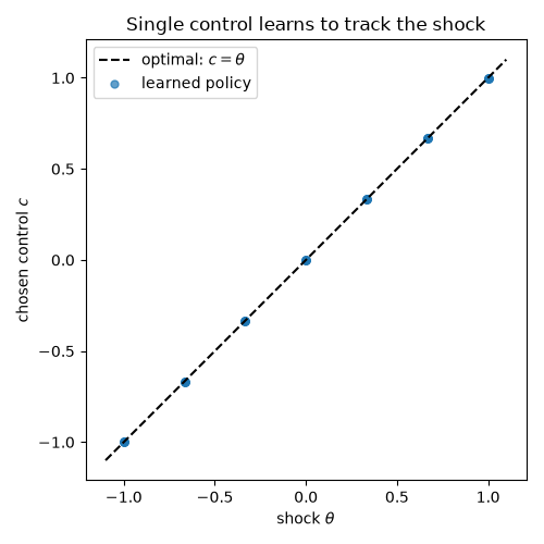
The agent observes a shock theta and chooses c. The reward \(u = -(\theta - c)^2\) is maximized when c equals theta, so the optimal decision rule is \(c(\theta) = \theta\). The control’s information set ["a", "theta"] lets the policy see the shock.

calibration = {"beta": 0.9}

b = block.DBlock(
    name="track the shock",
    shocks={"theta": (Normal, {"mu": 0, "sigma": 1})},
    dynamics={
        "c": block.Control(["a", "theta"]),
        "a": lambda a, c, theta: a - c + theta,
        "u": lambda theta, c: -((theta - c) ** 2),
    },
    reward={"u": "consumer"},
)
bp = bellman.BellmanPeriod(b, "beta", calibration)

Train over a grid of arrival states a and shock realizations theta. We use StaticRewardLoss, the negative of this period’s reward — the most direct single-period objective. (It reads each shock from the grid by its base name, "theta".)

states = grid.Grid.from_config(
    {
        "a": {"min": 0, "max": 1, "count": 7},
        "theta": {"min": -1, "max": 1, "count": 7},
    }
)

policy = ann.BlockPolicyNet(bp, width=16)
loss_fn = loss.StaticRewardLoss(bp)
ann.train_block_nn(policy, states, loss_fn, epochs=500)

learned_c = (
    policy.decision_function({"a": states["a"]}, {"theta": states["theta"]}, {})["c"]
    .detach()
    .flatten()
    .cpu()
    .numpy()
)
theta = states["theta"].flatten().cpu().numpy()

The learned rule lies on the 45-degree line \(c = \theta\).

fig, ax = plt.subplots(figsize=(5, 5))
lim = [theta.min() - 0.1, theta.max() + 0.1]
ax.plot(lim, lim, "k--", label=r"optimal: $c = \theta$")
ax.scatter(theta, learned_c, s=25, alpha=0.7, label="learned policy")
ax.set_xlabel(r"shock $\theta$")
ax.set_ylabel("chosen control $c$")
ax.set_title("Single control learns to track the shock")
ax.legend()
ax.set_aspect("equal")
fig.tight_layout()

Case 2: a block with two controls

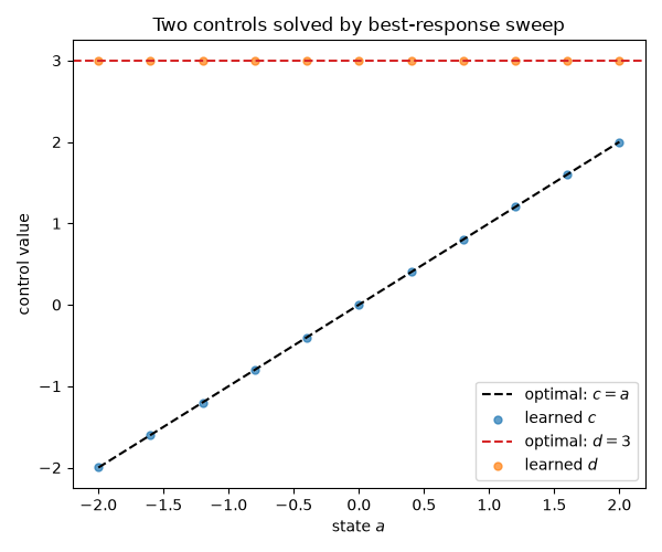
Here the reward \(u = -(a - c)^2 - (k - d)^2\) couples two controls. The optimum is \(c = a\) and \(d = k = 3\). The control d has an empty information set, so its optimal value is a constant.

torch.manual_seed(SEED)
np.random.seed(SEED)

multi_calibration = {"k": 3, "beta": 0.9}

b2 = block.DBlock(
    name="two controls",
    dynamics={
        "c": block.Control(["a"], agent="agent"),
        "d": block.Control([], agent="agent"),
        "u": lambda a, c, d, k: -((a - c) ** 2) - (k - d) ** 2,
    },
    reward={"u": "agent"},
)
bp2 = bellman.BellmanPeriod(b2, "beta", multi_calibration)

multi_states = grid.Grid.from_config({"a": {"min": -2, "max": 2, "count": 11}})

solve_in_order() solves the controls in the order given, each treating the others’ current policies as fixed, and NeuralBestResponse trains a network for each one. Repeating a symbol in the order list schedules an extra refinement pass for it.

method = NeuralBestResponse(
    GroundedBlock(b2, multi_calibration), multi_states, epochs=200
)
decision_rules = solve_in_order(method, ["c", "d", "c"])

a_vals = multi_states["a"].flatten()
c_vals = decision_rules["c"](a_vals).detach().cpu().numpy()
# ``d`` has an empty information set, so its rule takes no arguments: it returns
# one value per grid point using the length baked in by the solver.
d_vals = decision_rules["d"]().detach().cpu().numpy()
a_np = a_vals.cpu().numpy()

/home/runner/work/scikit-agent/scikit-agent/.venv/lib/python3.12/site-packages/torch/nn/modules/linear.py:124: UserWarning: Initializing zero-element tensors is a no-op
  init.kaiming_uniform_(self.weight, a=math.sqrt(5))

Both controls recover their optima: c follows a and d sits at the constant k = 3.

fig, ax = plt.subplots(figsize=(6, 5))
ax.plot(a_np, a_np, "k--", label="optimal: $c = a$")
ax.scatter(a_np, c_vals, s=25, alpha=0.7, label="learned $c$")
ax.axhline(3, color="C3", ls="--", label="optimal: $d = 3$")
ax.scatter(a_np, d_vals, s=25, alpha=0.7, color="C1", label="learned $d$")
ax.set_xlabel("state $a$")
ax.set_ylabel("control value")
ax.set_title("Two controls solved by best-response sweep")
ax.legend()
fig.tight_layout()

The residual reward confirms convergence: with the optimal policy the reward u should be approximately zero everywhere.

rewards = bp2.reward_function(
    {"a": a_vals},
    {},
    parameters=multi_calibration,
    decision_rules=decision_rules,
)
print(f"max |u| over the grid: {float(rewards['u'].abs().max()):.2e}")

plt.show()

/home/runner/work/scikit-agent/scikit-agent/examples/algorithms/plot_direct_block_solve.py:179: UserWarning: Converting a tensor with requires_grad=True to a scalar may lead to unexpected behavior.
Consider using tensor.detach() first. (Triggered internally at /__w/pytorch/pytorch/torch/csrc/autograd/generated/python_variable_methods.cpp:820.)
  print(f"max |u| over the grid: {float(rewards['u'].abs().max()):.2e}")
max |u| over the grid: 1.48e-04