PPO via Stable-Baselines3 on the D-4 Benchmark

This example shows how to solve a scikit-agent model with Proximal Policy Optimization (PPO), a deep reinforcement-learning algorithm. Rather than re-implementing PPO, scikit-agent wraps a BellmanPeriod in a gymnasium environment and hands it to the robust PPO implementation in Stable-Baselines3 (SB3). The PPOAgent class manages this wrapping, trains the agent, and emits a standard scikit-agent decision rule.

We test it on the D-4 benchmark: a deterministic, impatient CRRA consumption-savings problem with a binding borrowing constraint \(c_t \leq m_t\) (no borrowing). Unlike the perfect-foresight D-2 model, D-4 has no closed-form solution — the binding constraint kinks the consumption function — so we validate the learned policy against a numerical value-function-iteration (VFI) reference. This is precisely the setting where a general-purpose RL solver earns its keep: no model-specific structure is available to exploit.

Model Structure

• State variable: \(a_t\) — assets carried into period \(t\).

• Information variable: \(m_t = a_t R + y\) — cash-on-hand.

• Control variable: \(c_t\) — consumption, bounded by the borrowing constraint \(10^{-3} \leq c_t \leq m_t\). The agent cannot borrow, so consumption can never exceed cash-on-hand.

The agent maximizes expected discounted CRRA utility,

\[\max_{\{c_t\}} \; \mathbb{E}_0 \sum_{t=0}^{\infty} \beta^t \, \frac{c_t^{1-\sigma}}{1-\sigma}, \qquad a_{t+1} = (a_t + y - c_t) R .\]

Why No Closed Form

D-4 is calibrated to be impatient: \(\beta R = 0.9568 < 1\), so the agent would like to front-load consumption and borrow against future income — but the constraint \(c_t \leq m_t\) forbids it. The constraint therefore binds at low wealth, where the agent consumes all its cash-on-hand (\(c_t = m_t\)), and only slackens at higher wealth. This kink rules out the linear-in-wealth closed form that D-2 enjoys, so there is no analytical policy to compare against.

Instead we use skagent.models.benchmarks.d4_vfi_reference_policy(), an independent numerical oracle that solves the model by value-function iteration on a dense cash-on-hand grid. Because it is expensive, we solve it once up front and interpolate the resulting policy wherever we need it below.

Note

The main limitation of the SB3 integration is that PPO uses a constant discount factor gamma. It does not handle dynamic (state-dependent) discounting out of the box, so models with a non-constant discount variable are not yet supported by this path.

import matplotlib.pyplot as plt
import numpy as np
import torch

from skagent.algos.sb3 import PPOAgent
from skagent.bellman import BellmanPeriod
from skagent.distributions import Uniform
from skagent.env import discounted_rollout_reward
from skagent.models.benchmarks import (
    d4_block,
    d4_calibration,
    d4_vfi_reference_policy,
)

Configuration

We snapshot the learned consumption function at a few cumulative training-timestep counts so we can watch PPO close in on the optimum.

SEED = 0
CHECKPOINTS = [70_000, 90_000, 130_000]
MAX_EPISODE_STEPS = 200
N_EVAL_ROLLOUTS = 50
EVAL_ROLLOUT_STEPS = 200
INITIAL_A_LOW = 0.01
INITIAL_A_HIGH = 5.0

print("D-4 calibration:")
for param, value in d4_calibration.items():
    print(f"  {param}: {value}")

D-4 calibration:
  DiscFac: 0.92
  R: 1.04
  CRRA: 2.0
  y: 1.0
  description: D-4: Deterministic CRRA with binding borrowing constraint (no closed form)

The VFI Reference Policy

Because D-4 has no closed form, we solve it numerically with skagent.models.benchmarks.d4_vfi_reference_policy(). Each call runs a full value-function iteration, so we evaluate it once on a dense cash-on-hand grid and wrap the result in a cheap interpolant. This same reference policy serves both the grid comparison and the rollouts below. The VFI oracle is keyed on the arrival state \(a\), so we invert \(m = aR + y\) to query it on a grid of cash-on-hand values.

_REF_M = np.linspace(0.5, 10.0, 200, dtype=np.float32)
_REF_A = (_REF_M - d4_calibration["y"]) / d4_calibration["R"]
_REF_C = (
    d4_vfi_reference_policy({"a": _REF_A}, {}, d4_calibration)["c"]
    .detach()
    .cpu()
    .numpy()
    .astype(np.float32)
)


def reference_c(m):
    """Interpolate the precomputed VFI reference consumption at cash-on-hand ``m``."""
    m_arr = np.asarray(m, dtype=np.float32).reshape(-1)
    return np.interp(m_arr, _REF_M, _REF_C).astype(np.float32)


def reference_decision_rule():
    """Wrap the precomputed VFI reference as a skagent decision rule."""
    return {"c": lambda m: torch.as_tensor(reference_c(m))}

Build the Environment and Agent

A BellmanPeriod packages the D-4 block together with its discount variable and calibration. PPOAgent wraps it in a gymnasium environment and sets up SB3’s PPO; the discount factor gamma defaults to the model’s DiscFac. We sample initial assets uniformly so the agent sees a range of starting states during training.

bp = BellmanPeriod(d4_block, "DiscFac", d4_calibration)
initial = {"a": Uniform(low=INITIAL_A_LOW, high=INITIAL_A_HIGH)}

agent = PPOAgent(
    bp,
    initial,
    max_episode_steps=MAX_EPISODE_STEPS,
    seed=SEED,
    ppo_kwargs={
        "n_steps": 2048,
        "batch_size": 64,
        "n_epochs": 10,
        "learning_rate": 3e-4,
    },
)

Train PPO Incrementally

We train in stages, taking a frozen snapshot() of the policy at each checkpoint. reset_num_timesteps=False keeps PPO’s internal step counter (and learning-rate schedule) continuous across successive learn calls. The snapshots are unaffected by later training, so we can compare each one’s policy and rollout performance afterwards.

m_grid = np.linspace(0.5, 10.0, 41, dtype=np.float32)
obs_grid = m_grid.reshape(-1, 1)
snapshots = {}
c_learned_by_checkpoint = {}
prev = 0
for i, checkpoint in enumerate(CHECKPOINTS):
    print(f"Training up to {checkpoint:,} timesteps...")
    agent.learn(total_timesteps=checkpoint - prev, reset_num_timesteps=(i == 0))
    snapshots[checkpoint] = agent.snapshot()
    c_learned_by_checkpoint[checkpoint] = snapshots[checkpoint].predict_unscaled(
        obs_grid
    )
    prev = checkpoint

total_timesteps = CHECKPOINTS[-1]
episode_rewards = np.asarray(agent.episode_rewards, dtype=np.float32)

Training up to 70,000 timesteps...
Training up to 90,000 timesteps...
Training up to 130,000 timesteps...

Compare Against the VFI Reference

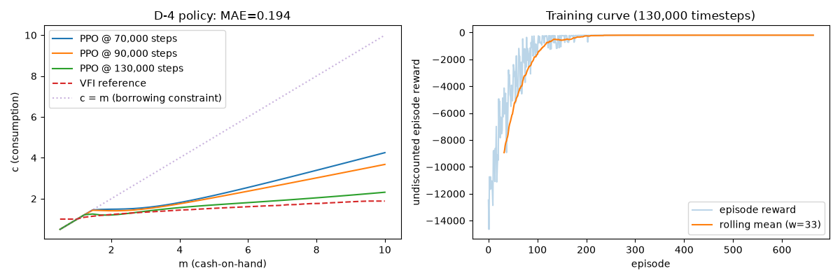
We evaluate the precomputed VFI reference policy on the same grid. At low cash-on-hand the borrowing constraint binds and the reference tracks the \(c = m\) line (the agent consumes everything); at higher wealth the constraint slackens and consumption falls below \(m\) as the agent saves.

c_optimal = reference_c(m_grid)

print(f"Policy error vs VFI reference (over m ∈ [{m_grid[0]}, {m_grid[-1]}]):")
print(f"  {'checkpoint':>12}  {'MAE':>10}  {'MaxErr':>10}")
mae_by_checkpoint = {}
for checkpoint in CHECKPOINTS:
    err = np.abs(c_learned_by_checkpoint[checkpoint] - c_optimal)
    mae_by_checkpoint[checkpoint] = float(np.mean(err))
    print(f"  {checkpoint:>12,}  {np.mean(err):>10.4f}  {np.max(err):>10.4f}")
mae = mae_by_checkpoint[CHECKPOINTS[-1]]

Policy error vs VFI reference (over m ∈ [0.5, 10.0]):
    checkpoint         MAE      MaxErr
        70,000      0.9241      2.3684
        90,000      0.7245      1.7932
       130,000      0.1937      0.5005

Visualize the Results

The left panel shows the learned consumption function at each checkpoint converging toward the VFI reference. The right panel shows the undiscounted episode reward over training, with a rolling mean to highlight the trend.

fig, axes = plt.subplots(1, 2, figsize=(12, 4))

for checkpoint in CHECKPOINTS:
    axes[0].plot(
        m_grid,
        c_learned_by_checkpoint[checkpoint],
        label=f"PPO @ {checkpoint:,} steps",
    )
axes[0].plot(m_grid, c_optimal, label="VFI reference", linestyle="--")
axes[0].plot(
    m_grid, m_grid, label="c = m (borrowing constraint)", linestyle=":", alpha=0.5
)
axes[0].set_xlabel("m (cash-on-hand)")
axes[0].set_ylabel("c (consumption)")
axes[0].set_title(f"D-4 policy: MAE={mae:.3f}")
axes[0].legend()

if len(episode_rewards) > 0:
    window = max(1, len(episode_rewards) // 20)
    rolling = np.convolve(episode_rewards, np.ones(window) / window, mode="valid")
    axes[1].plot(episode_rewards, alpha=0.3, label="episode reward")
    axes[1].plot(
        np.arange(window - 1, len(episode_rewards)),
        rolling,
        label=f"rolling mean (w={window})",
    )
    axes[1].set_xlabel("episode")
    axes[1].set_ylabel("undiscounted episode reward")
    axes[1].set_title(f"Training curve ({total_timesteps:,} timesteps)")
    axes[1].legend()
else:
    axes[1].set_title("No episodes completed during training")

fig.tight_layout()
plt.show()

Discounted-Reward Monte-Carlo Comparison

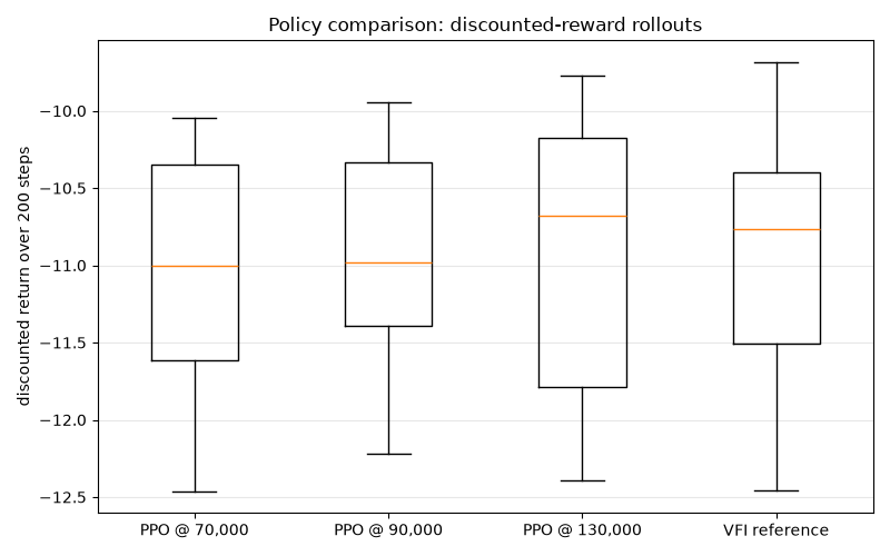
We also score the policies by their realized discounted return over many rollouts, comparing all three checkpoints against the VFI reference. Each checkpoint’s frozen snapshot exposes a decision_rule directly, so the rollouts use the exact trained policies — no reconstruction needed.

rng = np.random.default_rng(SEED + 1)
returns_by_policy = {}
for checkpoint in CHECKPOINTS:
    dr = snapshots[checkpoint].decision_rule()
    returns_by_policy[f"PPO @ {checkpoint:,}"] = [
        discounted_rollout_reward(bp, dr, initial, EVAL_ROLLOUT_STEPS, rng)
        for _ in range(N_EVAL_ROLLOUTS)
    ]
returns_by_policy["VFI reference"] = [
    discounted_rollout_reward(
        bp, reference_decision_rule(), initial, EVAL_ROLLOUT_STEPS, rng
    )
    for _ in range(N_EVAL_ROLLOUTS)
]

print(
    f"Discounted return over {EVAL_ROLLOUT_STEPS} steps "
    f"({N_EVAL_ROLLOUTS} rollouts each):"
)
for label, returns in returns_by_policy.items():
    print(f"  {label:>16}: mean = {np.mean(returns):8.4f}  std = {np.std(returns):.4f}")

Discounted return over 200 steps (50 rollouts each):
      PPO @ 70,000: mean = -11.0474  std = 0.7669
      PPO @ 90,000: mean = -10.9381  std = 0.6109
     PPO @ 130,000: mean = -10.9324  std = 0.8777
     VFI reference: mean = -10.9244  std = 0.8227

The boxplots summarize the distribution of discounted returns for each policy. As training progresses, the PPO return distribution shifts toward the VFI-reference benchmark on the right.

labels = list(returns_by_policy)
fig2, ax = plt.subplots(figsize=(8, 5))
ax.boxplot([returns_by_policy[k] for k in labels])
ax.set_xticks(range(1, len(labels) + 1))
ax.set_xticklabels(labels)
ax.set_ylabel(f"discounted return over {EVAL_ROLLOUT_STEPS} steps")
ax.set_title("Policy comparison: discounted-reward rollouts")
ax.grid(True, axis="y", alpha=0.3)
fig2.tight_layout()
plt.show()

Takeaways

PPO learns a consumption policy that tracks the VFI reference reasonably well — hugging the c = m borrowing constraint at low wealth and saving at high wealth — and the gap in discounted return shrinks across checkpoints, even though no model-specific structure was supplied to the solver. D-4 has no closed-form solution, so this is exactly the regime where the SB3 integration is most useful: a general-purpose baseline for models an analytical method cannot reach.