Lemons: Adverse Selection, and Three Markets That Look Alike

A seller knows what their own car is worth. A buyer does not, and can offer only what the average car on the market is worth. Every seller holding a car better than that average would rather keep it, so the good cars leave; the average falls; more sellers withdraw. Akerlof (1970) [1] showed that this can run all the way down, until nothing trades at all, even though every car is worth more to a buyer than to the person holding it.

What adverse selection is

Adverse selection is what happens when one side of a trade knows something about the good that the other side does not, and the terms on offer therefore decide which goods are brought to market. The uninformed side can price only an average, and an average price is most attractive to whoever holds the goods that are worst, so what trades is worse than what exists and the average the price was based on was the wrong one.

This market is that mechanism with nothing else in it. A seller knows \(\theta\) and a buyer does not, so the price can reflect only the average quality of the cars actually offered. Every seller whose car is worth more than the price keeps it, so the cars offered at price \(p\) are those with \(\theta \leq p\) and their average quality is below the average of the population. A buyer paying a premium on that lower average offers less than \(p\), fewer sellers are then willing, and the average falls again. The selection is visible in the model as the gap between the average car and the average car that trades, and the page measures that gap below.

This page does four things:

1. states the model and the price that clears it,

2. watches the market collapse, and checks the path against the closed form,

3. replaces the spread of quality with Akerlof’s two types, where the market has somewhere to stop, and

4. asks the analysis layer which of these markets can be solved one decision at a time.

The fourth is the reason there are several markets on this page rather than one. They are the same market under different timings, they have the same equations, and a cyclicity test cannot tell them apart – yet one needs an equilibrium solver, one needs only a simulation, and one is solved by backward induction.

The Model

Notation

• Shock: \(\theta_i\), the quality of the car seller \(i\) holds, which only that seller can see.

• Control: \(S_i\), whether to offer it, the one decision a seller makes.

• Price: \(p\), common to the whole market.

• Payoff: \(u_i\), the seller’s surplus, which is zero unless it sells.

A seller values a car at its quality and a buyer values it at a premium \(m\) on that quality, so a seller offers exactly when the price covers what the car is worth to them, and competition among buyers drives the price to the buyer valuation of what is actually on the market:

\[S_i = 1 \iff p \geq \theta_i, \qquad u_i = S_i (p - \theta_i), \qquad p = m \, E[\theta_i \mid S_i = 1]\]

The defaults are the paper’s own: quality uniform on \([0, 2]\), and a premium of \(3/2\).

Where the collapse comes from

Sellers offer when \(\theta \leq p\), so the cars on the market are uniform on \([0, p]\) and their average quality is \(p/2\). The price that clears is then \(m p / 2\), which for \(m = 3/2\) is \(0.75\,p\) – lower than the price the sellers were responding to. Repeat, and the market walks down to zero.

The map \(p \mapsto m\,E[\theta \mid \theta \leq p]\) has two readings. Iterated, it is the price path of a market whose sellers respond to whatever was posted last round. Read once, it gives the price that sellers anticipating \(p\) would bring about, so the prices it leaves unchanged are the equilibria of a market with no lag in it.

Three timings

The module composes the same blocks three ways, and the order is the whole of the difference:

• lemons_block: the sellers decide, the market clears on what they offered, and they are paid at that price. Nothing is lagged, so a seller’s rule has to anticipate the price that rule itself induces. This is a fixed point in rules.

• naive_lemons_block: the sellers are paid at a price already posted, and the market then clears at what their decisions imply. The price is read before it is written, so it is an arrival state and simulating the model is the iteration.

• monopsony_block: a single buyer names the price before any car is offered. The price is a decision, and the model is solved by backward induction.

References

[1]

Akerlof, G. A. (1970). “The Market for ‘Lemons’: Quality Uncertainty and the Market Mechanism.” The Quarterly Journal of Economics, 84(3), 488-500. https://doi.org/10.2307/1879431

import matplotlib.pyplot as plt
import numpy as np

import skagent.models.lemons as lemons
from skagent.ground import GroundedBlock
from skagent.simulation.monte_carlo import Simulator
from skagent.solver import project
from skagent.utils import plot_block_diagram


SELLERS = 20000
ROUNDS = 24

# Colours chosen for colour-vision deficiency: blue, vermilion, bluish green.
SERIES = ["#0072B2", "#D55E00", "#009E73"]


def posted_path(block, calibration, start, rounds=ROUNDS):
    """Simulate a posted-price market, and return the price after each round."""
    sim = Simulator(
        calibration,
        block,
        {"S": lemons.seller_rule},
        {"p": start},
        sample_count=1,
        T_sim=rounds,
        seed=0,
    )
    sim.initialize_sim()
    return np.asarray(sim.simulate()["p"]).ravel()

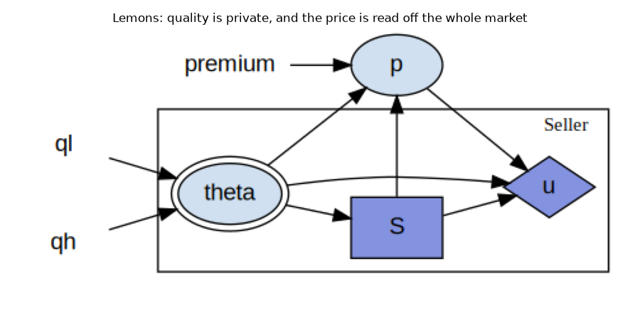
The model as the library sees it

The dynamics of the anticipated-price market, in the order they run. theta is the quality the seller holds, S the decision to offer it, p the price the market clears at, and u the seller’s surplus.

lemons.lemons_block.display_formulas()

S = Control(theta)
p = Function(theta, S, premium)
u = lambda S, p, theta: S * (p - theta)}

A decision carries the agent it belongs to and the information set it is taken on. The seller’s information set is its own car and nothing else, which is what makes the quality private and the market a lemons market:

for symbol, control in lemons.lemons_block.get_controls().items():
    print(f"decision {symbol:3s} agent {control.agent:8s} observes {control.iset}")
for symbol, agent in lemons.lemons_block.reward.items():
    print(f"payoff   {symbol:3s} agent {agent}")

decision S   agent seller   observes ['theta']
payoff   u   agent seller

The markets on this page are the same leaf blocks composed in different orders. Where the payoff block sits says which price a seller is paid at, and where the market block sits says whether the price is known when the seller decides, so the composition is the whole of the timing:

for label, block in [
    ("anticipated", lemons.lemons_block),
    ("posted price", lemons.naive_lemons_block),
    ("buyer commits", lemons.monopsony_block),
]:
    parts = []
    for part in block.blocks:
        inner = getattr(part, "blocks", None)
        parts.append(
            f"{part.name}({', '.join(b.name for b in inner)})" if inner else part.name
        )
    print(f"{label:14} {' -> '.join(parts)}")

anticipated    sellers(quality, supply) -> market -> payoffs(seller_payoff)
posted price   sellers(quality, offer) -> payoffs(seller_payoff) -> market
buyer commits  bid -> sellers(quality, offer) -> payoffs(seller_payoff) -> surplus

The model as a graph

Quality theta is a shock, the offer S is the seller’s decision, and u is the seller’s surplus. The one edge that leaves the seller class is the price p, which is read out of the whole population and paid to each seller individually. A single decision node stands for the class, which is what makes this a population model rather than a market written out one seller at a time.

market = GroundedBlock(lemons.lemons_block, lemons.lemons_calibration(size=SELLERS))

plot_block_diagram(
    lemons.lemons_block,
    "Lemons: quality is private, and the price is read off the whole market",
    calibration=market.calibration,
    figsize=(9, 4.5),
)

The selection, measured

At any price, the cars offered are the ones worth less than it, so the average car on the market is worse than the average car in existence. The gap between those two averages is the adverse selection, and the last column is what a buyer paying a premium on the offered average is willing to pay next.

print(
    f"{'price':>7} {'offered':>9} {'avg car':>9} {'avg offered':>13} {'clears at':>11}"
)
for price in (2.0, 1.5, 1.0, 0.5):
    sim = Simulator(
        market.calibration,
        lemons.naive_lemons_block,
        {"S": lemons.seller_rule},
        {"p": price},
        sample_count=1,
        T_sim=1,
        seed=0,
    )
    sim.initialize_sim()
    history = sim.simulate()
    quality = np.asarray(history["theta"]).ravel()
    offered = np.asarray(history["S"]).ravel() > 0.5
    print(
        f"{price:7.2f} {offered.mean():9.2%} {quality.mean():9.3f} "
        f"{quality[offered].mean():13.3f} "
        f"{float(np.asarray(history['p']).ravel()[0]):11.3f}"
    )

price   offered   avg car   avg offered   clears at
 2.00   100.00%     1.005         1.005       1.508
 1.50    74.80%     1.005         0.755       1.133
 1.00    49.66%     1.005         0.505       0.757
 0.50    24.46%     1.005         0.247       0.370

Every row clears below the price it started from, which is what walks the market down, and the table separates the two reasons for it. At a price of 2.0 every car is offered and there is no selection at all; the price falls anyway, because a buyer paying three halves of the average car values it at 1.508 rather than 2.0. Below that, selection appears and strengthens as the price drops: at 1.0 the cars offered average half of what the population does, and at 0.5 a quarter. The first effect starts the market falling and the second keeps it falling.

Three markets and their clearing maps

The figure below plots each market’s clearing map against the 45-degree line. Wherever the two cross, the price reproduces itself, and that is an equilibrium. The slope at a crossing says whether a market nearby moves toward it or away.

The three panels are the paper’s own market, the same market with a floor under quality, and the two-type market of the next section.

CONFIGS = [
    ("Akerlof's market\nquality uniform on [0, 2]", lemons.MARKETS["akerlof"], None),
    (
        "With a quality floor\nno car worth less than 0.4",
        lemons.MARKETS["partial-collapse"],
        None,
    ),
    (
        "Peaches and lemons\n70% of cars are peaches",
        lemons.PEACH_MARKETS["two-prices"],
        "two-type",
    ),
]


grid = np.linspace(0, 2.6, 400)
fig, axes = plt.subplots(1, 3, figsize=(12, 4), sharex=True, sharey=True)

for ax, (title, config, kind) in zip(axes, CONFIGS):
    if kind == "two-type":
        curve = np.array([lemons.peaches_clearing_map(p, **config) for p in grid])
        fixed = lemons.peaches_fixed_points(**config)
    else:
        curve = np.array([lemons.clearing_map(p, **config) for p in grid])
        fixed = lemons.clearing_fixed_points(**config)

    # These maps step where the worst car first becomes worth offering. Blanking
    # the point just past a step stops the line being drawn across it, which
    # would show prices the market never clears at.
    curve[np.abs(np.diff(curve, prepend=curve[0])) > 0.15] = np.nan

    ax.plot(grid, grid, color="0.7", linestyle="--", linewidth=1.5, zorder=1)
    ax.plot(grid, curve, color=SERIES[0], linewidth=2, zorder=2)
    ax.scatter(fixed, fixed, s=55, color=SERIES[1], zorder=3)
    for point in fixed:
        ax.annotate(
            f"{point:.2f}",
            (point, point),
            textcoords="offset points",
            xytext=(11, 7),
            fontsize=9,
            color="0.25",
            # The labels sit where the map meets the 45-degree line, so they are
            # lifted off both rather than printed over them.
            bbox={"facecolor": "white", "edgecolor": "none", "alpha": 0.8, "pad": 1},
        )
    ax.set_title(title, fontsize=10)
    ax.set_xlabel("price sellers respond to")
    ax.grid(True, alpha=0.25, linewidth=0.6)
    ax.set_axisbelow(True)

axes[0].set_ylabel("price the market then clears at")
axes[0].annotate(
    "45°",
    (2.1, 2.1),
    textcoords="offset points",
    xytext=(-4, 8),
    color="0.55",
    fontsize=9,
    rotation=38,
)
fig.suptitle("Where each market reproduces its own price", fontsize=12)
fig.tight_layout()

The left panel is the paper’s result. The map is a straight line of slope \(m/2 = 0.75\) through the origin, so it meets the 45-degree line only at zero, and no trade is the market’s one equilibrium.

A uniform range makes that line exactly straight, which is worth noticing, because it means the only prices such a market can reproduce are zero, a corner, or – if the premium were exactly 2 – every price at once. The two other panels are the two ways out of that.

The middle panel puts a floor under quality: no car is worth less than 0.4. The map is the same shape, lifted, so it crosses the 45-degree line at \(m\ell/(2-m) = 1.2\). Adverse selection still destroys the top of the market and the bottom keeps trading.

Watching a market walk down

Simulating naive_lemons_block runs one round of the map per period, so the price column of the history is the path. Three starting prices per market:

fig, axes = plt.subplots(1, 3, figsize=(12, 4), sharex=True, sharey=True)
starts = [2.0, 1.0, 0.3]

for ax, (title, config, kind) in zip(axes, CONFIGS):
    if kind == "two-type":
        block = lemons.naive_peaches_block
        calibration = lemons.peaches_calibration(size=SELLERS, **config)
    else:
        block = lemons.naive_lemons_block
        calibration = lemons.lemons_calibration(size=SELLERS, **config)

    for start, colour in zip(starts, SERIES):
        # Round 0 is the price posted before any of it happened, so the first
        # segment is the market's first response rather than an unexplained gap.
        path = np.concatenate([[start], posted_path(block, calibration, start)])
        ax.plot(
            np.arange(len(path)),
            path,
            color=colour,
            linewidth=2,
            label=f"start {start}",
        )
    ax.set_title(title, fontsize=10)
    ax.set_xlabel("round")
    ax.grid(True, alpha=0.25, linewidth=0.6)
    ax.set_axisbelow(True)

axes[0].set_ylabel("clearing price")
axes[0].legend(frameon=False, fontsize=9)
fig.suptitle("Where each market ends up, and what it started from", fontsize=12)
fig.tight_layout()

Peaches and lemons

The right-hand panels are Akerlof’s automobiles rather than a spread of quality: a car is a peach or a lemon and nothing between. That is a different market from the uniform one, and the difference is not a matter of degree.

Between a lemon’s worth and a peach’s, the only cars offered are lemons, and their average quality is a lemon’s worth however many peaches exist. So the clearing map is flat there, and it crosses the 45-degree line at \(m\ell\). Trade survives, and every peach is withheld. Above a peach’s worth every car is offered, and the price is the premium on the average car, which reproduces itself if peaches are common enough to carry it.

The result is three basins in one market. Where it ends up depends on where it started, which is something none of the other models in this library ask of a solution concept.

config = lemons.PEACH_MARKETS["two-prices"]
print(f"a lemon is worth 0.4 and a peach 2.0, and {config['share']:.0%} are peaches")
print()
print(f"prices this market reproduces : {lemons.peaches_fixed_points(**config)}")
print(f"peaches trade only above      : {lemons.peach_share_for_trade():.4f}")
print()
for start in starts:
    path = posted_path(
        lemons.naive_peaches_block,
        lemons.peaches_calibration(size=SELLERS, **config),
        start,
    )
    print(f"  started at {start:<4} -> {path[-1]:.4f}")

a lemon is worth 0.4 and a peach 2.0, and 70% are peaches

prices this market reproduces : (0.0, 0.6000000000000001, 2.2800000000000002)
peaches trade only above      : 0.5833

  started at 2.0  -> 2.2814
  started at 1.0  -> 0.6000
  started at 0.3  -> 0.0000

Below that critical share, no price a buyer will pay for the average car is enough to bring a peach out, and a market that starts high still falls back to the lemons:

scarce = lemons.PEACH_MARKETS["lemons-only"]
path = posted_path(
    lemons.naive_peaches_block,
    lemons.peaches_calibration(size=SELLERS, **scarce),
    2.5,
)
print(f"only {scarce['share']:.0%} peaches, started at 2.5 -> {path[-1]:.4f}")

only 30% peaches, started at 2.5 -> 0.6000

Which of these can be solved one decision at a time?

A solver needs to know whether the decisions in a model fall into an order. The relevance graph answers that: its nodes are decisions and its edges say which decision has to account for which. If the graph is acyclic, the decisions can be settled one at a time, in order.

Asked about the class as it is declared, the graph separates the four versions of this market:

MARKETS_TO_CHECK = [
    ("anticipated", lemons.lemons_block, lemons.lemons_calibration(size=SELLERS)),
    (
        "posted price",
        lemons.naive_lemons_block,
        lemons.lemons_calibration(size=SELLERS),
    ),
    (
        "peaches, anticipated",
        lemons.peaches_block,
        lemons.peaches_calibration(size=SELLERS),
    ),
    ("buyer commits", lemons.monopsony_block, lemons.lemons_calibration(size=SELLERS)),
]


def report(rows):
    """One row per market: its decisions, what relies on what, and the verdict.

    A reliance that holds across the instances of a class is named with the
    class in brackets, since on the class's own symbol it is a self-loop and the
    shape alone would not say so.
    """
    print(f"{'market':22} {'decisions':28} {'relies on':42} solvable in order")
    for label, graph in rows:
        edges = [
            f"{a} -> {b}"
            + (f" [{graph.plate(a).entity}]" if graph.crosses_instances(a, b) else "")
            for a, b in graph.edges()
        ]
        answer = "yes" if graph.is_acyclic() else "no"
        relies = ", ".join(edges) or "(none)"
        print(f"{label:22} {', '.join(graph.nodes()):28} {relies:42} {answer}")


report(
    [
        (label, block.relevance_graph(calibration))
        for label, block, calibration in MARKETS_TO_CHECK
    ]
)

market                 decisions                    relies on                                  solvable in order
anticipated            S                            S -> S [seller]                            no
posted price           S                            (none)                                     yes
peaches, anticipated   S                            S -> S [seller]                            no
buyer commits          p, S                         p -> S                                     yes

The two anticipated markets report the sell decision as relying on itself, across the seller class: a seller’s payoff runs through the price to every other seller’s decision, so what is wanted is one rule that is its own best response rather than a step in an order. What the bracket in that column reads off is crosses_instances(), beside plate(), which names the class and its size – Plate(entity='seller', size=20000) here. In the posted-price market the same decision relies on nothing, and that is correct, because that period’s payoff turns on the previous round’s price and within a round there is nothing to account for. The two blocks differ only in where the payoff block sits.

One symbol cannot refer to another instance of itself, so that reliance is derived on a split of the class – one node for the seller being solved, one for the rest of it – which is what project() builds. Asked of the projection directly, the same reliance is a pair of edges between the two sides:

def projected_graph(block, calibration):
    projected = project(GroundedBlock(block, calibration))
    return projected.block.relevance_graph(projected.calibration)


report(
    [
        (label, projected_graph(block, calibration))
        for label, block, calibration in MARKETS_TO_CHECK
    ]
)

market                 decisions                    relies on                                  solvable in order
anticipated            S_other, S_actor             S_other -> S_actor, S_actor -> S_other     no
posted price           S_other, S_actor             (none)                                     yes
peaches, anticipated   S_other, S_actor             S_other -> S_actor, S_actor -> S_other     no
buyer commits          p, S_other, S_actor          p -> S_other, p -> S_actor                 yes

The self-loop in the first report is that pair read back onto the class’s own symbol, so the two reports say the same thing about each market.

The two anticipated markets have edges in both directions between the seller being solved and the rest of the class: each has to account for the other, and the component is cyclic. These are the markets that need an equilibrium.

The posted-price market has no edges even after the split, because the price its sellers respond to was set before the round began. Simulating it is enough.

The market where a buyer commits has two edges, both from the price to the sellers, and no cycle. Its topological order is backward induction: solve the sellers against a price, then the buyer against the sellers.