Incentives in Content Recommendation: Wanting Control Versus Having It

Content recommendation separates value of control from the instrumental control incentive. A recommender paid for clicks gains an incentive to change the user’s mind, and none at all to reach what they thought before arriving.

A recommender chooses posts from a model of a user’s opinions and is paid for clicks. Whether those clicks are the ones the influenced user actually produces, or ones predicted from the model of their original opinions – the one thing that differs between the two diagrams below – decides whether the recommender has an incentive to change the user’s mind at all. That is the difference between a variable merely being worth moving and the agent’s own decision being what moves it, and only the second is a hazard a design can be held responsible for. That hazard is manipulation: an agent paid for what its outputs do to people acquires an incentive to change them, which nobody wrote into its objective, and preventing that is what the variation below is for.

Both diagrams come from Everitt, Carey, Langlois, Ortega and Legg [1] and are encoded as blocks in skagent.models.safety.incentives, with the criteria read off the diagram by skagent.relevance before any payoff is chosen and without solving anything. The companion page, Incentives in Grade Prediction: Observing Versus Responding, develops the other pair of criteria.

References

[1] (1,2)

Everitt, T., Carey, R., Langlois, E., Ortega, P. A. and Legg, S. (2021). “Agent Incentives: A Causal Perspective.” AAAI-21, 35(13), 11487-11495. arXiv:2102.01685.

[2]

The graphical tests are Theorems 16 and 18 of [1], for value of control and the instrumental control incentive. Both are sound and complete, so an answer read off the diagram holds for every way of filling in the numbers.

import matplotlib.pyplot as plt
import numpy as np
from skagent.models.safety.incentives import (
    content_recommender_block,
    content_recommender_redesign_block,
    draw_shocks,
    print_incentive_table,
)
from skagent.utils import plot_block_diagram

The Model

A recommender chooses which posts to serve, P, on the basis of a model M it holds of a user’s original opinions O. The posts it serves go on to influence those opinions, I. Clicks C are what it is paid for, and they depend both on the posts and on the user’s opinions as the posts have left them.

plot_block_diagram(
    content_recommender_block,
    "Content recommendation: clicks depend on the influenced opinions",
)

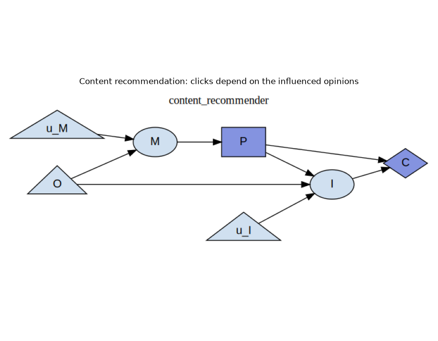
The block carries one node more than the diagram as usually drawn, per chance mechanism: the exogenous noise that writing each mechanism in structural-causal form makes explicit. Those are the u_ names, and they are filtered out of the tables below.

Value of Control, and the Instrumental Control Incentive

Writing \(\pi\) for the recommender’s rule for choosing posts, the value of control in a variable \(X\) is the payoff gained by being able to set \(X\) rather than take it as it comes – to choose it with a rule \(g\) of its own, from whatever \(X\) already depends on:

\[\mathrm{VoC}(X) \;=\; \max_{\pi,\, g} \mathbb{E}\big[C\big] \;-\; \max_{\pi} \mathbb{E}\big[C\big].\]

An instrumental control incentive in \(X\) is a different thing: payoff flowing through \(X\), so that freezing \(X\) at the value it would have taken under some reference decision \(p_0\), while the recommender goes on varying its posts, changes what it earns,

\[\mathbb{E}\big[C \mid \mathrm{do}(P = p)\big] \;\neq\; \mathbb{E}\big[C \mid \mathrm{do}(P = p),\; \mathrm{do}(I = I(p_0))\big].\]

Value of control asks whether a variable would be worth moving by anyone; an instrumental control incentive asks whether the agent’s own decision is what moves it. Both are decided from the diagram alone, by admits_voc() and admits_ici() [2].

print_incentive_table(content_recommender_block, criteria=("VoC", "ICI"))

 node   VoC   ICI
    C   yes   yes
    I   yes   yes
    M   yes     -
    O   yes     -
    P   n/a   yes

SCIM(7 nodes, 8 edges, decisions=['P'])

Two rows carry the argument.

The first is I, the influenced opinions, which admits an instrumental control incentive. What that amounts to on the diagram is a directed path running from the decision through I and on to the payoff, and what it means here is that the recommender is paid for what its posts do to the user’s opinions. Nobody wrote that objective down. It is implied by paying for clicks in a world where posts change minds, and it is the manipulation incentive.

The second is O, the user’s original opinions, which admits positive value of control and no instrumental control incentive at all. The recommender would gain from setting what the user thought before it ever arrived, and it has no way to reach back and do so. That is an idle wish rather than a hazard, and it is where the two criteria part company.

The Variation

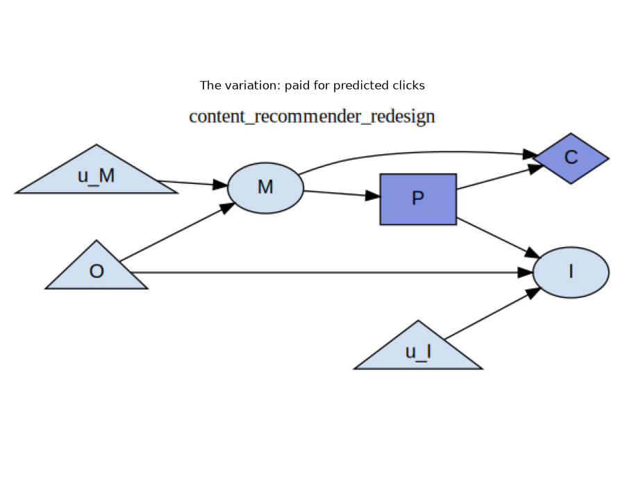
The payoff is retargeted. The recommender is paid for clicks predicted from its model of the user’s original opinions, rather than for the clicks the influenced user actually goes on to produce. It still chooses posts, those posts still influence opinions, and it is still paid for a click-shaped quantity; only which quantity has changed.

plot_block_diagram(
    content_recommender_redesign_block,
    "The variation: paid for predicted clicks",
)

print_incentive_table(content_recommender_redesign_block, criteria=("VoC", "ICI"))

 node   VoC   ICI
    C   yes   yes
    I     -     -
    M   yes     -
    O   yes     -
    P   n/a   yes

SCIM(7 nodes, 8 edges, decisions=['P'])

I now admits neither. Nothing directed leaves it any more, so no path from the decision can reach the payoff through it, which means the manipulation incentive is gone and the value of controlling the user’s opinions has gone with it. That is the point of the variation: the harm was removed by changing what the recommender is paid for, not by asking it to behave. O keeps its value of control and still admits no instrumental control incentive, exactly as before: retargeting the payoff did not put the user’s past within reach.

Checking It Against the Mechanisms

This is the second display above, evaluated. Hold the influenced opinions at the value they would have taken under a baseline recommendation \(p_0 = 0.5\), let the recommender vary its posts anyway, and compare what it earns against what it earns when opinions are free to respond.

posts = np.linspace(0.0, 1.0, 21)
baseline_post = 0.5

fig, axes = plt.subplots(1, 2, figsize=(12, 5), sharey=True)
panels = [
    (content_recommender_block, "paid for actual clicks", axes[0]),
    (content_recommender_redesign_block, "paid for predicted clicks", axes[1]),
]

for block, title, axis in panels:
    block, shocks = draw_shocks(block, n=50_000)
    frozen_opinions = block.transition(shocks, {"P": lambda M: baseline_post})["I"]

    responsive, frozen = [], []
    for post in posts:
        responsive.append(block.transition(shocks, {"P": lambda M: post})["C"].mean())
        frozen.append(
            block.transition(
                {**shocks, "I": frozen_opinions}, {"P": lambda M: post}, fix=["I"]
            )["C"].mean()
        )

    axis.plot(posts, responsive, linewidth=2, label="opinions respond to the posts")
    axis.plot(
        posts, frozen, linewidth=2, linestyle="--", label="opinions held at baseline"
    )
    axis.set_xlabel("P — post intensity")
    axis.set_title(title)
    axis.grid(True, alpha=0.3)
    axis.legend()

axes[0].set_ylabel("expected payoff")
plt.tight_layout()
plt.show()

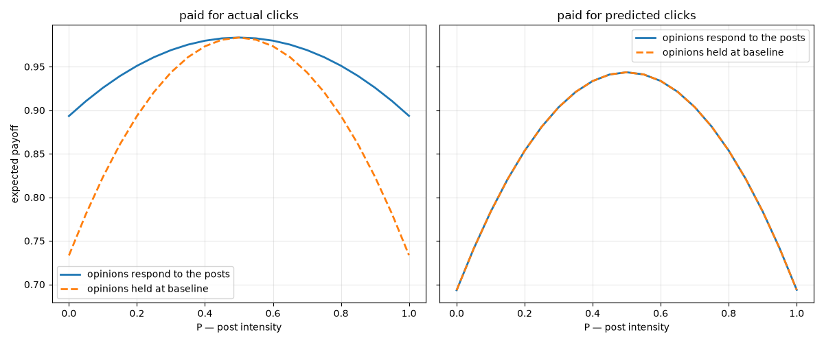
On the left the two curves come apart everywhere except at the baseline post itself, where freezing the opinions changes nothing by construction. Away from it, a recommender paid for actual clicks earns more, because the opinions have moved toward whatever it posted. That gap is the payoff flowing through the user’s mind, and it is what the instrumental control incentive on I names. On the right the curves coincide at every post, because the retargeted payoff never reads the influenced opinions, so freezing them costs nothing. That is the incentive’s absence, made numerical.

What the Criteria Cost

Both tables on this page were computed from the graph alone, with no payoff values, no distributions and no solving. The numeric check came afterwards, and it confirmed what the graph had already said. That order is the point, because it means the criteria can screen a design before it is built, and a criterion that answers “no” rules the behaviour out for every way of filling in the numbers.

The direction in which these tests err is worth knowing. Soundness and completeness are properties of the diagram, and d-separation is conservative on the deterministic mechanisms these blocks are written with, so an incentive may be reported in a case where the functional effect happens to vanish. The converse cannot happen. A criterion here may cry wolf, but it will not miss one.