Note
Go to the end to download the full example code.
Mean-Field Equilibrium: Solving for an Economy’s Capital
When an economy is made of many small agents, each one takes the economy’s aggregates as given. A household in the Aiyagari economy [1] does not reckon that its own saving moves the interest rate, since its saving is one part in thousands of the capital stock. Each household solves a problem in which the capital stock, and the prices that follow from it, are numbers handed to it. The economy is in a mean-field equilibrium when the capital those households’ saving adds up to is the capital they were handed.
The Aiyagari page of the model gallery builds the economy and checks its simulation against a closed form under a fixed savings rule. This page takes the households’ saving as a choice and solves for it. It uses that economy without re-deriving it, so read that page for the model.
This page does four things:
states the equilibrium as a fixed point in one number, the capital stock,
projects the economy onto one household’s problem at a given capital stock, and solves it,
finds the capital stock at which the economy reproduces itself, and
varies the income risk, and checks the answer against the economy without it.
Setup
The household’s discount factor is 0.96. We fix the dispersion of the endowment at \(\sigma = 0.3\) for the first three steps.
import matplotlib.pyplot as plt
import numpy as np

import skagent.models.aiyagari as aiyagari
from skagent.ground import GroundedBlock
from skagent.solver import (
    ExactStationaryBestResponse,
    project_mean_field,
    solve_mean_field,
)
from skagent.utils import plot_block_diagram


BETA = 0.96
SIGMA = 0.3
HOUSEHOLDS = 1000

# Colours chosen for colour-vision deficiency: blue, vermilion, bluish green.
SERIES = ["#0072B2", "#D55E00", "#009E73"]


def economy(sigma):
    """The Aiyagari economy at income risk *sigma*, as the full model."""
    return GroundedBlock(
        aiyagari.aiyagari_block,
        {
            **aiyagari.aiyagari_calibration(size=HOUSEHOLDS, sigma=sigma),
            "DiscFac": BETA,
        },
    )
The economy without income risk
One value anchors everything below. If no household faced income risk, a single representative household would hold all the capital, and it would save until the interest rate equalled its rate of time preference, \(R = 1/\beta - 1\). Since \(R = \alpha K^{\alpha-1} - \delta\), that fixes the capital stock:
Aiyagari’s point is that income risk makes households save more than this, to insure against bad draws, so the economy’s capital should lie above \(K_{RA}\).
K_RA = (aiyagari.CAPITAL_SHARE / (1 / BETA - 1 + aiyagari.DEPRECIATION)) ** (
    1 / (1 - aiyagari.CAPITAL_SHARE)
)
print(f"K_RA = {K_RA:.4f}")
K_RA = 5.4468
One household’s problem, at a given capital stock
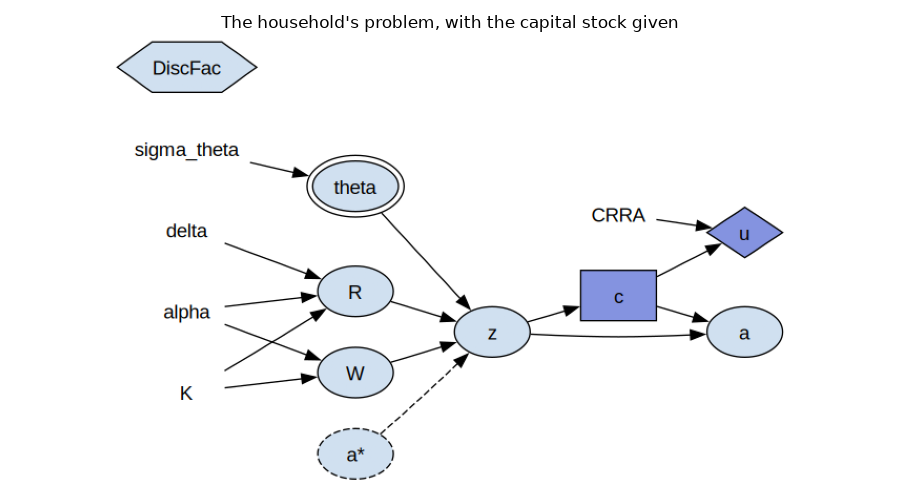
In the full model the capital stock \(K\) is computed from the households’
assets, so a household’s problem depends on every other household’s choice.
project_mean_field() cuts that dependence. It removes
the equation that averages the class, and leaves \(K\) a symbol the rest
of the model reads. What remains is the problem of a single household facing
prices it takes as given. Once \(K\) has a value, the diagram below shows
it as a parameter beside \(\alpha\) and \(\delta\), and the household
as a decision-maker alone.
population = economy(SIGMA)
projected = project_mean_field(population)

plot_block_diagram(
    projected.block,
    "The household's problem, with the capital stock given",
    calibration={**projected.calibration, "K": K_RA},
    discount="DiscFac",
    figsize=(9, 5),
)
Solving it takes a method that finds the household’s stationary rule, the
one that is best forever rather than for one period.
ExactStationaryBestResponse does that by iterating
the Bellman operator on a grid of assets to its fixed point. The grid is
denser near zero, where the rule bends most, and
confine_to_grid=True keeps next period’s assets on it.
method = ExactStationaryBestResponse(
    projected,
    {"a": 60 * np.linspace(0, 1, 30) ** 2},
    "DiscFac",
    disc_params={"theta": {"N": 5}},
    confine_to_grid=True,
)
The capital stock enters through the prices. A larger stock lowers the interest rate and raises the wage. To see what that does to the household, solve the problem at two values of \(K\) and plot the consumption each rule gives at a range of cash on hand.
cash = np.linspace(0.5, 12, 200)

fig, ax = plt.subplots(figsize=(7, 4.5))
for K, color in zip((0.9 * K_RA, 1.1 * K_RA), SERIES[:2]):
    at_K = method.with_ground(projected.with_calibration({"K": K}))
    rule = at_K.best_response("c", {})
    ax.plot(cash, rule(cash), color=color, label=f"$K = {K:.2f}$")
ax.plot(cash, cash, color="grey", linestyle=":", label="consume everything")
ax.set_xlabel("cash on hand, $z$")
ax.set_ylabel("consumption, $c$")
ax.set_title("A household's saving rule at two capital stocks")
ax.legend()
fig.tight_layout()
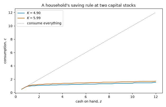
At the larger stock the wage is higher and the interest rate lower, and the household consumes more at every level of cash. Each curve is one household’s whole plan at that stock. Neither says which stock is the equilibrium one: for that, the households’ saving has to add up to the stock they were given.
The capital stock that reproduces itself
For a candidate stock, solve_mean_field() solves the
household’s problem as above, then simulates the full model, the one in which
\(K\) is the average of the households, under the resulting rule. The
simulation settles at some capital stock, \(K_{sim}(K)\), which in general
differs from the candidate. The difference is the residual, and the
equilibrium is where it is zero. Brent’s method finds that root, within a
bracket whose ends have residuals of opposite sign. Here the bracket runs from
\(K_{RA}\) upward, since risk can only raise saving.
rule, info = solve_mean_field(method, population, bracket=(K_RA, 1.1 * K_RA), tol=1e-3)
print(f"converged: {info['converged']} after {info['iterations']} iterations")
print(f"K = {info['aggregate']:.4f}, against K_RA = {K_RA:.4f}")
converged: True after 7 iterations
K = 5.5480, against K_RA = 5.4468
Every candidate the root-finder tried is in info["rounds"], with the stock
the simulation settled at. Plotting \(K_{sim}\) against the candidate shows
the map the root-finder worked on, and where it crosses the diagonal.
rounds = sorted(info["rounds"], key=lambda r: r["candidate"])
candidates = np.array([r["candidate"] for r in rounds])
simulated = np.array([r["simulated"] for r in rounds])

fig, ax = plt.subplots(figsize=(6, 5))
ax.plot(candidates, candidates, color="grey", linestyle=":", label="$K_{sim} = K$")
ax.plot(candidates, simulated, color=SERIES[0], marker="o", label="$K_{sim}(K)$")
ax.axvline(info["aggregate"], color=SERIES[1], linewidth=1, label="equilibrium")
ax.axvline(K_RA, color=SERIES[2], linewidth=1, linestyle="--", label="$K_{RA}$")
ax.set_xlabel("capital stock the households are given, $K$")
ax.set_ylabel("capital stock the economy settles at, $K_{sim}$")
ax.set_title("The economy's capital against the capital it was given")
ax.legend()
fig.tight_layout()
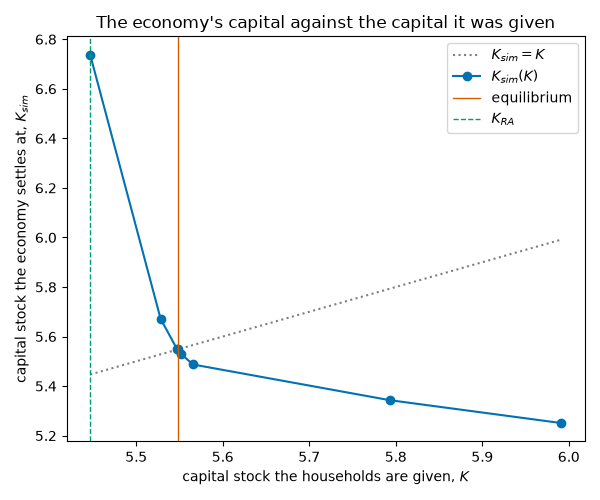
The map slopes downward. Handed a low stock, the interest rate is high and the households save a lot, so the economy ends up with more than it was given. Handed a high stock, the reverse. That is what lets a root exist, and it is why a bracket from \(K_{RA}\), where the economy overshoots, to a larger stock, where it falls short, contains the equilibrium.
The off_grid count in each round reports how many simulated households
held assets past the grid the household’s problem was solved on. It is zero
or a handful for every candidate up to a little above the root, and in the
hundreds for the largest ones, where the low interest rate sends households
to assets the grid does not cover. The rule is extended past its grid, so the
simulation runs, but a count that large says the answer at that candidate
is not to be trusted.
     K    K_sim  off grid
5.4468   6.7375         0
5.5283   5.6712         1
5.5475   5.5479         3
5.5480   5.5479         3
5.5523   5.5288         3
5.5654   5.4874         5
5.7929   5.3433       223
5.9915   5.2507       836
Income risk raises capital
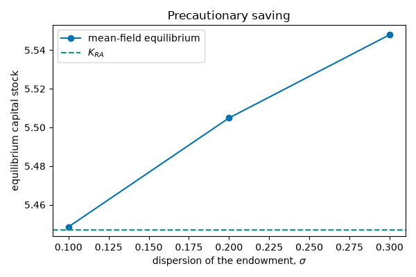
Repeating the solve at several dispersions of the endowment gives Aiyagari’s comparative static. Each solve is a separate economy, with its own projection and its own method.
sigmas = [0.1, 0.2, 0.3]
equilibria = {SIGMA: info["aggregate"]}
for sigma in sigmas:
    if sigma in equilibria:
        continue
    pop = economy(sigma)
    _rule, found = solve_mean_field(
        ExactStationaryBestResponse(
            project_mean_field(pop),
            {"a": 60 * np.linspace(0, 1, 30) ** 2},
            "DiscFac",
            disc_params={"theta": {"N": 5}},
            confine_to_grid=True,
        ),
        pop,
        bracket=(K_RA, 1.1 * K_RA),
        tol=1e-3,
    )
    equilibria[sigma] = found["aggregate"]

fig, ax = plt.subplots(figsize=(6, 4))
ax.plot(
    sigmas,
    [equilibria[s] for s in sigmas],
    color=SERIES[0],
    marker="o",
    label="mean-field equilibrium",
)
ax.axhline(K_RA, color=SERIES[2], linestyle="--", label="$K_{RA}$")
ax.set_xlabel(r"dispersion of the endowment, $\sigma$")
ax.set_ylabel("equilibrium capital stock")
ax.set_title("Precautionary saving")
ax.legend()
fig.tight_layout()

print(f"{'sigma':>7s}{'K':>9s}{'above K_RA':>12s}")
for sigma in sigmas:
    K = equilibria[sigma]
    print(f"{sigma:7.2f}{K:9.4f}{K / K_RA - 1:12.2%}")
sigma        K  above K_RA
 0.10   5.4485       0.03%
 0.20   5.5049       1.07%
 0.30   5.5480       1.86%
At the smallest dispersion the economy is within a fraction of a percent of the representative agent’s, which is the check that the solver agrees with the closed form where one exists. The gap then widens with the risk: households save more as their income becomes less certain, and the economy’s capital rises with them.
Where the method stops
Every household plays the one rule, so the equilibrium found is symmetric by construction, and the capital stock is read from a finite simulation, so it is pinned to the precision of the class size and not beyond. Both are properties of the mean-field concept and of this solver, not of the economy.
References
Total running time of the script: (1 minutes 38.028 seconds)